Document Modeling Details with SAS Enterprise Miner, Easily and Consistently

One recent (6 months) trend in financial services is that regulators have asked companies to document details of models submitted for review. Challenge many companies face is that many modelers, experienced or not, are often not very well skilled in document-writing. Document style, structure, standards... vary by the modelers, by job roles, by departments and sheer language skills, among others. 

There is one facility inside SAS Enterprise Miner (EM), however, that is becoming very popular in relieving the condition. The feature, the usage of Score Node and Reporter Node together, has actually been within EM for a long time. 

The picture below shows a moderately elaborate EM model project

The focus of this blog is the Score Node and Reporter Node, down right hand size. 

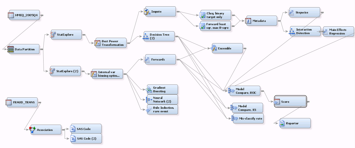
1. EM's Score node is listed under Assess tool category. While it normally performs SCORING activities, the goal of the scoring exercise in this flow context is NOT towards score-production. On the contrary, scoring here is often towards validation (especially one-off scoring on ad hoc testing data files for the model), profiling and, YES, reporting. Reporting is where this regulatory task falls under. 
2. You can link the Score to a model, or Model Comparison node as indicated by the picture above. 
3. The picture below shows how to click through to get to the Score node

Once the Score node is connected to a preceding model or Model Comparison node, you can click on the Score node to activate the configuration panel as shown below

1. For this reporting task, you can ignore details underneath Score Code Generation section. 
2. The selections under Score Data are important, but that is if you have partitioned the model data set into validation or test data set or both. You typically have at least one of them for regulatory reporting exercise.
3. You can test and see what are underneath the Train section.

Below shows how you click through to introduce the Reporter node to the flow. 

After you introduce the Reporter node and connect it to the Score node, the configuration panel, the core focus of this blog, appears upon clicking the node

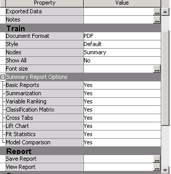
1. As of today, two Document formats are supported, PDF and RTF. RTF is a draft format for Word. Given that the direct output from EM Reporter node typically is used/perceived as a great starting pointing, subject to further editing using Word, not a final version, RTF format is more popular than PDF. Of course, if you prefer using Adobe for editing you can use PDF
2. There are four styles available, Analysis, Journal, Listing and Statistical. +four Nodes options, Predecessor, Path, All and Summary. So far, the most popular combination among banks is Statistical /Path. 
3. Selecting Show All does produce much more details. The resulting length of the document can easily exceed 200 pages.
4. You can configure details under Summary Report Options to suit your case. It is very flexible. 
5. This is how EM works: when you add nodes to build model, say, add EDA nodes like transformation and imputation, EM automatically records transformation and imputation, or 'actions'. When you connect a Score node, the Score node picks up all the details along the path (therefore the option Path or All Path), compile them into score code and flow code. The score code, in SAS data step, SAS programs (meaning procedures), (for some models) C, Java and PMML, is then available for production. When you add the Reporter node, EM will report on the process details.

To sum, the biggest advantage of using the Score +Reporter combination in EM is to provide one efficient, consistent starting model documentation template. Consistent because now if you ask the whole modeling team to report using the same set of configuration options, you get the same layout, granular details and content coverage. That is a big time saver. 

Thank you. 

From Wellesley, MA

Associative Rule Mining (ARM) using SAS In-Memory Statistics for Hadoop: A Start-up Example

In SAS Enterprise Miner, there are Market Basket Node and Association Node. In SAS In-Memory Statistics for Hadoop ("SASIMSH"), the statement ARM (Associative Rule Mining) covers most, if not all what the two nodes do inside Enterprise Miner. This post presents a start-up example on how to conduct ARM on SASIMSH. While it does not change much of  Market Basket Node and Association Node essentially do, you will see how fast SASIMSH can get the job done over 300 million rows of transaction over 12 months.

I focus on discussion of association based upon which, if you introduce temporal order of the transaction, you can easily extend /imagine into sequence.

The SASIMSH system used for this post is the same as the one used for my post dated 12/14/2014 "SAS High Performance Analytics and In-Memory Statistics for Hadoop: Two Genuine in-Memory Math Blades Working Together". Here are some info on the data set used.

The data set is simulated transaction data set consisting of 12 monthly transaction, 25 million transaction entries each, totaling 300 millions. The total size of the data set is ~125 GB. Below is monthly distribution.

T_weekday is how many transactions happen Sunday, Monday, Tuesday... Saturday. T_week counts how many transactions happen on week 1... week24....week52 on the year. These segment variables are created in case you want to break down your analysis.

Below is main body of the ARM modeling code

1. The two "Proc LASR" sections create LASR in-memory analytics process and load the analytics data set into it. The creation process took ~10 seconds and the loading process took ~15 seconds (see picture)

2. The Frequency statement simply profiles the variables the distributions of which I reported above.
3. The ARM statement  is where the core activities happen

•  Item= is where you list the variable of product category. You have full control product hierarchy.
•  Tran= is where you specify granular level of transaction data. There are ~9 million unique accounts for this exercise. If you choose to use a level that has, say, 260 unique level values (with proper corresponding product levels) you can easily turn the ARM facility into BI reporting tool, closer to IMSTAT's GROUPBY statement does.
• You can use MAXITEMs= (and/or  MINITEMS) to customize item counts for compilation
•  Freq = is simply order count of the item. While Freq = is more 'physical, accounting book weight'        (therefore less analytical, by definition), Weight= weighting is more analytical /intriguing. I used list price here, essentially compiling support  in terms of individual price importance, assuming away any differential price-item elasticity and a lot more. You can easily have a separate model to study this weight input alone, which is beyond the scope of this post. 
•  The two aggregation options allow you to decide how item aggregation and ID aggregation should happen; if weight = is left blank, both aggregations ignore the aggregation= values you plug in and aggregate by default value of SUM, which is really to ADD UP. Ideally, one aggregation should use one weight variable. For now, if you specify weight=, the weigh variable is used for both. If you are really so 'weight' sensitive, you can run the aggregation one at a time, which does not  much more time and resources.
•  The ITEMSTBL option asks  output of a temporary table to be created in-memory amid the flow for further actions during the in-memory process, the table system-reserved keyword  .&_tempARMItems_ refers to in the next step. This is different from what SAVE option generates. SAVE typically outputs table to Hadoop directory "when you are done".
•  The list of options commented out in GREEN show that you can customize support output; you don't have to follow the same configurations when the ARM model was being fit above when generating rules or association scores.

4. Below is how some output looks like

•  The _T_ table is the temporary table created. You can use PROMOTE statement to make it      permanent
•  _SetSize_ simply tells number of products in the combinations.
•  _Score_ is the result of your (double) aggregations. Since you can select one of 4 aggregation  
•  options (SUM, MEAN, MIN, MAX) for either aggregation (ITEMAGG and AGG), you need to interpret the score according to your options.

5. This whole, while sounding cliche content wise, takes only ~8 minutes to finish over 300 million rows.

The gap between CPU time and real time is pretty large, but I care less since the overall is only 8 minutes.

SAS High Performance Analytics and In-Memory Statistics for Hadoop: : Two Genuine in-Memory Math Blades Working Together

SAS In-Memory Statistics for Hadoop ("SASIMSH" ) and SAS High Performance Analytics Server (“SAS-HPA”) are two key in-memory advanced analytics /modeling products SAS Institute (“SI”) offers today. Both support Hadoop as data source server: SASIMSH is Hadoop centric while SAS-HPA supports Hadoop, Teradata and others. While both have its own in-memory data management capabilities, there are applications and efficiency scenarios where one is engaged to build out data sets to share between the two. 

This post shows how to integrate (modeling) data sets from local SAS clients, SASIMSH’s LASR server and HPA, with a Hadoop cluster (“the cluster”) serving as central data repository. Some performance details are also shown. 

1. The cluster and other system features

• The cluster has 192 nodes, with 96GB RAM each (CPU and other details on the individual nodes are unknown, but are of ‘2014 standard level’). Only 14 nodes are engaged for the exercises; all the performance details are conditional upon this many nodes
• All the performance details are with other users’ concurrent jobs running at the cluster
• The local SAS client is a virtual machine /cloud running 64-bit Windows  2008 R2 standard server with 32 GB RAM,  Intel Xeon(R) CPU, X7560 @2.27 GHz, 2.26 GHz (4 processors). Not that these details are critical. Just so you know. It has some relevance when you load data from traditional SAS sources onto LASR servers. Jobs running on the client have no other concurrent jobs running while reporting the performance details.

2. The action on LASR server 

In the picture ("Pic 1") above,

2.1 This is SAS Studio, not SAS Editor or SAS EG

2.1 "LIBNAME bank2": 
    2.11. SASHDAT is system reserved engine label, specifically indicating that the library being established and pointing to is a Hadoop file co-location. Explaining 'co-location' in great detail is beyond the scope of this post. For now, imagine Hadoop is where big data chunk is stored. SASIMSH and SAS-HPA are like (math) blades sitting along side Hadoop. Stick the blade into Hadoop, lift the data into memory, get the math job done and put results back to Hadoop if any (sometimes you just take the insights or score code without writing back to Hadoop)
   2.12. SERVER= is just your host. Path= CAN supports as many slashes/directory levels as you like. 

2.2 "LIBNAME bank3": just your regular SAS local directory.

2.3 "goport=1054": you pick a port number to ask for allocation of a slice of memory space (which in this case is collective, 96GB*14, -/~) for your action.  As of today, this number cannot exceed 65535 and must not have been reserved: if you just ran this port to create a LASR server with this port number, you (or somebody else) need to terminate that server to release the port number (and, YES, destroy everything you did within that previous in-memory session. You will see the benefits of doing so later) if you want to use the same number again. Of course you can use a different number, if it is available. A good (tactical) habit (with strategic implication for having a good life with in-memory analytics) is to use a limited set of numbers as ports. One obvious reason is that in memory like this is not to use the memory space to mainly store (the huge) data chunk. One logical, associated question therefore is how fast it is to load/reload (big) data chunk into LASR server from the client, or from the Hadoop co-location. ("if it takes forever to load this much, I have to park it". Sounds familiar?). You will see how fast it takes to load in both ways, shortly.

2.4 "outdsn=...; ": I declare a file location the library of which is yet to be set. That is not problem, as long as you set the library before eventually USING it. You can put everything between = sign and ; and it will not fail you.

2.5 "PROC LASR Create": This is to create a new LASR server process, with the port number. Path=/tmp is similar to temp space in regular SAS session. 

2.6 "Lifttime=7200": I want the server to cease in two hours.
2.7 "Node=all": all the 14 nodes available. Not the 192 nodes physically installed. Either your administrator caps you, or you can manually set Node=14. 

2.8 "PROC LASR Add": this is to load the data from Hadoop library BANK2 (the co-location) into the LASR server defined by the port number. 

The data set: 300 million rows, ~45 variables. 12 monthly transactions combined, 25 million rows/month. Total file ~125 GB. 

The WHERE statement conditions out the last 7 months while loading the input into memory. Note: there is no SAS Workspace in LASR operation. 

The picture below shows that the loading takes 6.54 seconds, most of which is CPU time. Which is desirable. Which implies 'data piping' and trafficking takes little time.

3. Load local data onto the LASR server

In the pic ("Pic 2") above,

3.1 "Libname bank22":  sasiola is system reserved label indicating that library BANK22 is a SAS LASR input-output (IO) LASR library. Plain English: use this engine/library to input SAS data sets from outside LASR library. TAG: this short-name option is key to handle file system like Hadoop where directory can easily breach the two-level limitation regular SAS library-data set can support. Within the quotes, the directory can have as many slashes or levels as needed.

3.2 "Data...": syntax wise, this is just regular SAS data steps. I am stacking the last 7 month data sets from two different local SAS libraries, Bank3 and Bank4. T_ is  least minimum action you should take to make additional analytical use of any date data you have in your data set. Most (not all) data steps in SAS BASE are supported.

As shown in the picture below, the log shows ~19 minutes of the loading act

The CPU time is not much, indicating piping and trafficking takes time. Considering this is loading from local C drive and D drive of the virtual machine Windows client, this is expected. Notice: the resulting 5 month file now resides in the same in-memory library Bank22. 

SASIOLA engine apparently is key gateway connecting traditional SAS data sourcing with in-memory LASR servers. However you have been building your data sets, you can load it to LASR server via SASIOLA. You can definitely originate your data sources directly within LASR.


4. Append /Stack data set in SASIMSH. 

The picture below ("Pic 3") shows how the two data sets, one directly loaded from Hadoop cluster, one loaded off local SAS,  are stacked using LASR server in-memory. 

4.1 Unlike SAS BASE steps, the table listed at the TABLE has to be one of existing tables; it is called ACTIVE table. The SET action here is defined as 'to modify the active table'. 

4.2 The table listed at SET statement to modify inherits the active table's library; as this version of SASIMSH stands, one has to load both tables into the same library to perform the act; spelling out library name in front of the data set name will cause error.

4.3 Drop option at SET statement is very nice considering you may very well be setting gigantic data onto the active table: YES, space management remains essential during in-memory analytics. 

And it takes, how long? 247 seconds.

4.4 "Save...": after the appending act is over, write the resulting 12 month data set back to Hadoop cluster. Copy and Replace are ordinary Hadoop options. (1 copy and replace existing file with the same name). Recall: the Hadoop cluster directory is where SAS-HPA picks up data for its operations. And the writing time is included within the 247 seconds elapsed. 

5. Terminate LASR server. After the work is done, the LASR server is terminated, as shown in the picture below.

Now you can launch HPA procedures such as HPSUMMARY to run additional analytics. 

Final notes:

• SAS-HPA has its own data management facilities such as HPDS2 that has strong OOP (Object Oriented Programming) orientation and flavor. Which is more native to traditional formats such as ANSI-SQL
• Both HPDS2 and SASIMSH support traditional SAS BASE step syntax, with a few exceptions. 
• There are use cases where you prefer parking large data set in ported LASR servers. For example, if, instead of stacking 7 monthly files, you are stacking 24 monthly files. That may take >>20, 18 minutes. You can conceivably stack the 24 data sets, share the port with others who want to consume the resulting one big data set. They just set proper library to access it. 
• The central philosophy of SASIMSH, by way of fast loading and clean termination, is that against the reality of data changing instantly and much, one may have desire to build more and more analytics in high pace. Be flashy. Classic such example is digital marketing analytics where input data are often live, highly interactive social event streams. 
• SASIMSH is resource sensitive. In another separate environment where 47 nodes with 96GB/ node, all steps were finished with a minute. 96GB RAM per node, by 2014 standard , is under par. Today the standard RAM equipped with each node is 512 GB, or at least 256 GB. If you want to read 2TB data from Hadoop, of course you need stronger and more node machines. As  practical matter, not a general statement, I have observed that virtual machines as node member on the cluster, run obviously more slowly than if the nodes are real, physical machines. 

SAS In-Memory Statistics for Hadoop: Using PROC IMSTAT to Transpose Data

SAS® In-Memory Statistics for Hadoop ("SASIMSH")  is a single interactive programming environment for analytics on Hadoop that  integrates analytical data preparation, exploration, modeling and deployment. It contains PROC IMSTAT and  SAS LASR Analytic Engine (SASIOLA). SASIOLA essentially is 'BASE' for SASIMSH, whereas PROC IMSTAT covers the full analytical cycle from BASE, through modeling, towards deployment. This duality continues SAS's long standing tradition of 'getting the same job done in different ways', to accommodate users' different style, constraints  and preferences.

This post is one of several upcoming posts I plan to publish soon that discuss code mapping of key analytical data exercises from traditional SAS programming to SASIMSH. This post today covers using PROC IMSTAT to transpose data.

Prior to IMSTAT being available, SAS users typically either write data step code or engage PROC transpose to transpose data. In PROC IMSTAT, PROC transpose is not supported (of course, because there is no way another procedure is supported to run underneath and within a procedure like PROC IMSTAT, or any SAS procedure. There is no statement in PROC IMSTAT to explicitly do what PROC transpose does either). However, PROC IMSTAT CAN be programmed to transpose. This post provides one such example. 

Code part 1: Set up in-memory analytics SAS libraries for Hadoop + loading

Below is code part 1 screen shot

• The first LIBNAME statement sets up library reference to a Hadoop cluster by the IP address  of sas.com (I cleaned up confidential address info), which I am using 14 parallel nodes out of >180 nodes in total. 
• At this design interface, the analyst (me) does not care if the underlying Hadoop is Cloudera or Horton Works or somebody else. IMSTAT is designed NOT to program differently simply because the underlying Hadoop is 'from a different flavor of Hadoop'. Bank2 is the name for the SAS library, as if you are just setting one up for regular SAS work or access to Oracle, Green Plum DB or Teradata DB. The naming convention is the same.
• SASHDAT is the quintessential differentiator for SAS in-memory advanced analytics. It appears just like regular SAS Access driver. It actually is, but much more in the interest of enabling genuine in-memory analytics; somebody can write a book about this 'driver' alone. For now, it simply allows us to enable SAS in-memory data access onto Hadoop. 
• Path= is a directory management structure, little new.
• From the DATA statement, 
• I am simulating 12 months of variable X data for 1 million IDs. Simple. 
• I am asking SAS to write the 12 million rows directly to Hadoop in the SASHDAT format. In doing so, I also request that the resulting data set &indsn be sorted by ID (the partition= data set option) and further sorted by MONTH (orderby=). The fact with 'sorting' in a parallel system like this, though, is that sorting (with the partition= option) is actually grouping: sorting by ID actually is just placing records with the same ID values together; they do not collate any more (meaning sequencing groups in descending or ascending value of the variable ID like BASE SAS is doing with PROC SORT) . Since later access to the grouped records will be parallel, why spending more time and resources ( a lot if your data set is huge) asking them to further collate after initial grouping? Orderby= option is to add collation WITHIN grouped groups. The notion of using partition= AND orderby= is the same with "PROC SORT; by ID month;", but the physiology and mechanism of the act is different, moving from a 'single server' mode to parallel world (or from SMP to MPP)
• Also, the partition and orderby options are supported as data set options (in a typical MPP Hadoop operation as such, likely these two data set options are only supported at output data sets, not at input data set. Why?), whereas in regular BASE SAS operation, the analyst has to call up separate PROC SORT to do it. This luxury is affordable now because this is IN-MEMORY, this is no longer disk swapping (Imagine more and you will enjoy this more, I promise)
• The Replace=: this is Hadoop finger print. If the destination library is set up to point to other DB such as ORACLE or Teradata, or any DBMS-like, this option does not work. As Hadoop is towards more 'managed' (not necessarily towards DBMS, but Yarn, Kerberos...) this may or may not change. Not shown here, but I recall another option is Copy=. The Copy option simply tells Hadoop how many copies it should make for the data set you are dumping into its laps. 

• At "PROC LASR", 
• This block is creating one in-memory working session by requesting allocation of port 10002 (if available at the time I submit the request) as "access, passing lane" to the server,  by requesting directory "/tmp" as "operating/temp parking ground'. 
• Lifetime =: tells IMSTAT that after 72000 seconds, trash the whole session and everything within it. Noclass=: not required, has something to do with categorical variable loading
• Performance nodes=ALL: means all Hadoop nodes that are available and policy-permitted by whoever is in charge of the 'box'
• The second "PROC LASR" has ADD option asking that the table I wrote to the target Hadoop cluster be loaded into the memory session I just created. As you may learn more and more about 'loading data into memory', this is only one of many loading methods.  The analyst, for example, certainly can load many SAS7BDAT data sets sourced by all kinds of traditional venues and practices (PROC SQL, BASE...) by using another in-memory engine SASIOLA. There are also data loader products from SAS as well. Once the table is loaded into memory, it parks there until the server is terminated. 
• Notice: this session implicitly inherits the server from previous lines, if not directed or specified otherwise. The port, however, must be explicit while trying to load data into it. The session is port specific and the port is generic: port number 10002 means the same to whoever is using it.

Code Piece 2: Reference the loaded file in-memory, build code to transpose

Below is code part 2 screen shot

• The LIBNAME TRANS engages SASIOLA engine to call up the file just loaded into the memory space by pointing to the directory where the in-memory session is set up. This LIBNAME statement uses tag= option to represent this reference for later processing. This tagging act is to respond to the fact Hadoop system typically has system of directories, which is worsen by the fact Hadoop systems often run off Linux-like OS which per se has limitless directories. Traditionally SAS products support two levels such as mysas.in. Tagging therefore is in place. 
• The "PROC FCMP" portion is entirely my doing that does not much to generalize. I show how one can generate code in this way. You can certainly type or copy to make your own reference code file. 
• The ARRAY details in the middle of FCMP should be straightforward. I am sure you can make it more sophisticated, implicit (or mysterious). The point is to show one basic approach to transpose data with IMSTAT. Noteworthy is the __first_in_partition and __last_in_partition. This is nothing but your familiar first.ID and last.ID. Their invocation certainly depends on the data set being partitioned/sorted (where did it happen in this post? Did it already happen?)

Code Piece 3: Using PROC IMSTAT to tranpose/score the data

Below is code part 2 screen shot

As many SAS users often say, the last piece is the easiest. Once the code is built, you can run it through the SCORE statement. To use the __first_in_partition and __last_in_partition, you MUST specify partition option value at the SCORE statement. In this way, IMSTAT will go search for the partition table created while partition= and orderby= options were effected (this certainly is not the only way to partition and order). FETCH is similar "PROC PRINT". 

The last "PROC LASR" with TERM is to terminate the in-memory session once the job is done. This is one important habit to have with SAS LASR centered in-memory analytics, although not a technical requirement. Lengthy discussion on this subject belongs to another post. 

Here are some log screen shots

Generating 12 Million Records, 3 Variables, 14 Seconds

Load 12 Million Records, 3 Variable to Memory, 2.6 Seconds

 

Transposing takes 5 Seconds

TRANSPOSED !

October 2014, from Brookline, Massachusetts 

SAS In-Memory Statistics (IMSTAT) for Hadoop Overview

SAS® In-Memory Statistics for Hadoop ("SASIMSH")  is a single interactive programming environment for analytics on Hadoop that  integrates analytical data preparation, exploration, modeling and deployment. It contains PROC IMSTAT and  SAS LASR Analytic Engine (SASIOLA). SASIOLA essentially is 'BASE' for SASIMSH, whereas PROC IMSTAT covers the full analytical cycle from BASE, through modeling, towards deployment. This duality continues SAS's long standing tradition of 'getting the same job done in different ways', to accommodate users' different style, constraints  and preferences.

This post provides overview of IMSTAT, with a little associated coverage of the SASIOLA facilities. 

You certainly read through IMSTAT details here at sas.com. Below is a summary picture many have liked better, to capture features and functions of PROC IMSTAT. It covers the latest as of Q1 of 2014, but the spirit and gist remain the same since.

Some comments about the 'total concept' first
1. If you are familiar with SAS products and solutions, you are used to seeing BASE (programming), STAT (statistical sciences), ETS (Econometrics), OR (operations research), EM (enterprise data mining including machine learning, text mining and statistics), EG (enterprise guide) and MM (model management). Another line of SAS in-memory products still largely follow this set of convention. For example, HP Statistics (high performance counterpart of STAT), HPDM (high performance counterpart of EM) and so on. You are used to seeing long list of procedures under each product or package. 

Now, conceptual 'shock' #1 is all these features listed in this IMSTAT picture are grouped under ONE procedure. Yes, IMSTAT is one procedure and one procedure only, with so many features

2. Why this change?

If you use any of the traditional SAS products mentioned above, you know to get the work on hand done, you likely engage a very small set of procedures, functions and statements afforded by a specific product that you have license for. For example, I myself have been using STAT since ~1991, but still ~ half of the procedures under STAT remain stranger to me. I don't recall having known anybody who uses all of the BASE capabilities either. On the contrary, I know friends who have held SAS jobs for many years. They are experienced, but have only known just half a dozen procedures.
The reality though is it is not cost possible for a software developer to build just a few procedures for one company and build another small set for another company.

One way SAS has to address this (price and value) gap is software on demand offerings, in-depth discussion of which is beyond the scope of this post. Another way is to redesign package in such a way that all the essential features and functions to get analytical jobs done are built in and integrated. The next immediate question is: which to pick and chose from which existing packages? Apparently, from elementary 'can do' perspective, it is hard to imagine many things that SAS cannot do with its existing offerings. In many cases, the challenge is how, not if. Still, a coherent organizing theme is needed to build the new piece. Good news is such piece has existed for many years.

The BLUE spoke in the center of the picture presents a diagram of modern analytical life cycle, from problem definition, data preparation and exploration, through modeling, to deployment and presentation. PROC IMSTAT features and functions are organized and developed by this framework. In other words, PROC IMSTAT has collected core functions and features from SAS software families, to optimize against needs and challenges confronting analytical users in Hadoop world. Many 'pre-existing' features have been distilled and streamlined while being moved to the in-memory platform. 

PROC IMSTAT is expanding rapidly to accommodate ever changing Hadoop world.

Some comments about PROC IMSTAT
1. Major pure feature and function addition actually are on the right side, the recommender engine. Everything else essentially has been in existence in SAS software family in some format or style.
2. All the entries listed under a box header label (such as Data Management to the top left corner) are IMSTAT statements. To access the statements, the user must invoke "PROC IMSTAT" first. Unlike many traditional SAS procedures where one has to invoke procedures many times, once PROC IMSTAT is invoked once, the user can invoke the same statement again and again, as the job deems necessary
3. User who are very familiar and deep on some SAS procedures may find that some features, reduced from a regular SAS procedure (for example, CORR statement stems from PROC CORR) to IMSTAT statement, no longer have that many options as their counterpart procedures have. This, in part, is because the procedure has been reduced to a statement. Another reason is more strategic design; the reduction or left-out is intentional: do you really think it makes sense to run all those distance options under the cluster statement on now much bigger data sets?
4. Some statements actually are mini-solution.  GroupBy statement, for example, is "in-memory cube builder " or a genuine OLAP killer, while it appears like a small statement

I plan to publish specific use case to help better understand how IMSTAT works. Thanks.

October 2014, from Wellesley, Massachusetts 

SAS High Performance Finite Mixture Modeling, HPFMM: Introduction by One Example

SAS Institute released HPFMM procedure with its High Performance Statistics 13.1, after the regular FMM procedure was made available through regular STAT package for years.

This post is not intended to show or discuss how to do FMM. A solid, yet simple discussion of FMM with excellent SAS concentration can be found in professor Malthouse's book. There is also a excellent blog on regular FMM procedure usage. A SAS developer of the FMM procedure also did a video on FMM.

This post is to showcase computational  power of the new HPFMM procedure over the regular FMM procedure. For those who have little exposure to FMM practice, but need to compute on bigger data sets with the method, this post covers essential aspects to get on with FMM, since regular PROC FMM and HPFMM overlap a lot.

This is the first time I have used the new SAS Studio to build blogs here. I will cover some SAS Studio as well.

Introduction

1. What is FMM: in plain English, "a variable is distributed in such fashion you believe it is mixture of components"
2. How FMM varies, to name a few ways,
1. By component type: categorical, interval... leading to very different governing/underlying distributions. One sub-direction in this vein is observed or unobserved where you can find intellectual connections to some canonical analysis
2. By interrelationship among components: same variance, mean?
3. By if and how mixing interacts with components: share covariates? determine / estimate simultaneously?
4. how 'weird' the distorted distribution is: you can fit and match to several major, if not popular 'skewed' distribution class such as zero inflation, Poisson distribution.

Description of data set used for the post

1. 5 million observations, 204 variables. The response variable is binary Y/N, with 'response rate' ~26.76% or 1,338,111=Y. Response is B2C Q & A: "Do you have your desired product now?"
2. The 204 variables are mostly RFM variables dating back to the past 72 months, + some attributes. 

The environment the SAS HPFMM job is running on:

1. A 192-node Cloudera Hadoop Cluster with SAS HP STAT 13.1 loaded. The specific job is capped at 14 nodes, with each node having >96 GB ? (this number is not important, given this size of the data). FMM rarely has real time or near real time requirement; running faster than what is shown in the post likely does not provide much incremental value.
2. The job is conducted using SAS HP STAT 13.2, the latest version of the software
3. The coding is through a virtual Windows client machine with 32 GB local RAM. The client connects to the Hadoop  cluster. No FMM processing happens locally on the client.

The code and the editing interface, the new SAS Studio


Running HPFMM at SAS Studio

• This is the look of SAS Studio which essentially is SAS enhanced editor, but represents a revolutionary leap-forward from its ancestors in classic SAS Enhanced Editor, Enterprise Guide, or Enterprise Miner. The Studio is web-native, built for collaboration and portability and 'flashy'. It is much better at output rendering, log, message and error handling, and version management + the modern touch and feel. In current analytics world when look does matter sometimes, the Studio is a true contender in stability, integrity, consistency and support.
• If you are familiar with SAS procedure programming, the program does not present much surprises; if you are familiar with PROC FMM, you can plug in your existing program, add the Performance statement and start tweaking. If you are just learning how to use SAS FMM facility, starting with PROC FMM and PROC HPFMM should provide similar learning return in speed, functionality and feature, with some exceptions (which you probably don't care)

Still some notes,

• The default Output statement setting is no longer copying all the variables over from the input data set, especially any input variable and BY variables, unlike the regular PROC FMM where all are moved over to output data set listed at OUTPUT statement, if ID statement is not engaged. This is rather a contrast between all the HP procedures and their non-HP counterparts, not just with the FMM procedures.
• The default maximum iteration is set at 200 or maximum function calls at 2000. I raised them to 5000 and 250000 respectively, just to test, not to suggest the simplex optimization method requires that. As some of you may have experienced, another factor in tweaking is link function. The point here is: if called for, more iterations and function calls now can be handled with the HPFMM procedure fairly quickly
• What does not converge under PROC FMM probably still does not converge under HPFMM, eventually. So, exploratory data analysis, design, business domain, prior or posterior knowledge about the model project remain quintessential for success. 
• Rules of thumb such as "identity link runs much faster than other links" probably still hold, everything else being equal, as far as I have tested. 

The HPFMM log,

1. You can set message level to get more details. 
2. Three traffic lights on top left corner indicate summarily how the program goes.
3. Carrying ~200 variables into the process with 5 million records (yes, I deliberately decided not to write Keep= or Drop = statement to shrink input variable list, because the time spent on writing that code likely exceeds the time taken to finish the entire job without dropping them, the 27-28 second mark), it finished below 28 seconds. 
4. The gap between CPU time and Real time is still large, percentage wise, but I care less since it is in seconds, unlike regular SAS session where the gap may be in minutes or hours
5. This is genuine in-memory computation in which the data set is loaded into memory residing with the 14 nodes on the target Hadoop cluster. Once the job is done, data are dropped off the memory space. The resulting output data set, as I wished and specified, is written to the cluster
6. When using PROC FMM, tackling 5 million rows with 200 + variables is harder to manage; on the 32 GB Windows machine where this blog is being typed right now, I cannot have PROC FMM to finish the job. I have to cut the data set down to the short list of variables to make it through. And it took > 16 minutes. 
7. Overall, you still need to be data efficient. If you have, say, >600K variables (a near reality where a lot of text/unstructured elements are involved in modeling <not necessarily FMM>), you may still consider Keep/Drop variables. 

FMM output, the administrative section,

1. Count of Hadoop nodes involved in the job is first reported
2. You then see link function details. Some modelers disrespect identity. Well, in this specific case, I have tested, in a total of 10 minutes, that three other link functions do NOT provide better results any way. Respect what the data have to tell you, because IDENTITY is the fastest
3. All the estimation / convergence is now ML
4. The class variable details should be exciting simply because now you are running on full sample in so little time. 

HPFMM output, the estimation section, 

1. The fit statistics and Z value, pretty straight forward. You can read all the books to appreciate underpinning definitions and rules; I am not sure I am qualified to profess you on the technicalities here (I don't have Ph.D title) 
2. One cautionary note: keep in mind these are computed statistic. Always interpret and use them with the specific data condition in mind. They may not be as 'portable' as you think, which blunt the motivation many decide to leverage mixture modeling, to begin with.

FMM output, the performance section (sort of),

1. The probability estimate serves as a direction as to how 'well' the model is. Data some time defy what numbers you should put in as K value (or range thereof). In some cases, you have to 'insist' or 'hold on' to your K value even if data support 'better' mixing probabilities otherwise
2. Professor Malthouse's book, aforementioned, provides great examples using PROC KDE and PROC SGPLOT to assist with K value insights. KDE on large data set can also be practiced with another SAS in-memory product IMSTAT (the KDE statement there) and SAS Visual Analytics (VA). 

Thank you.

Autumn of 2014, from Chestnut Hill, Massachusetts

SAS In-Memory Statistics for Hadoop: Key Exercises to Jump-Start Long Time SAS Users, Part One

SAS® In-Memory Statistics for Hadoop ("SASIMSH")  is a single interactive programming environment for analytics on Hadoop that  integrates analytical data preparation, exploration, modeling and deployment. It contains PROC IMSTAT and  SAS LASR Analytic Engine (SASIOLA). SASIOLA essentially is 'BASE' for SASIMSH, whereas PROC IMSTAT covers the full analytical cycle from BASE, through modeling, towards deployment. This duality continues SAS's long standing tradition of 'getting the same job done in different ways', to accommodate users' different style, constraints  and preferences.

This post is one of several upcoming posts I plan to publish soon that discuss code mapping of key analytical data exercises from traditional SAS programming to SASIMSH. This post today covers sorting, sorting related BY and ordering in SASIMSH.

Almost every modeler/analyst who has ever prepared data for modeling using SAS tools is familiar with PROC SORT, Set By on the sorted data set and/or further engaging first. and last. processing.

In SASIMSH, "Proc Sort" is NO LONGER explicitly supported as syntax invocation. However, the act of sorting is definitely supported. The naming/syntax invocation is now changed to PARTITION. Below are two code examples

Example 1 : partition under SASIOLA engine

" libname dlq SASIOLA START TAG=data2;
       data dlq.in(partition=(key2) orderby=(month) replace=yes);
          set trans.dlq_month1
                trans.dlq_month2;
       run; "

1.  At the LIBNAME statement, specification of SASIOLA continues the spirit of SAS Access drivers; you probably have run SAS Access to Oracle or older versions of SAS like V8 at LIBNAME statements before.  The option START is unique with SASIOLA (IOLA standing for input-output LASR). It simply tells SAS to launch the SASIOLA in-memory server (you can release the library or shut down the server later) . TAG= is critical and is required. One reason is to reference the data properly once it is loaded into the memory.  Another,  associated, reason is to avoid potential 'collision' when multiple actions are happening in the memory space. Also, when loading data from, say, Hadoop where the source has many layers of locations, the two-level restriction embedded with traditional BASE is no longer sufficient. Tag will allow for long specification.
2. SET statement can still be used to stack data sets . Still, there is no limit as to how many data sets you can stack; salient concern is sizing: how much memory space  is needed to accommodate the input data sets combined, a concern you care far less when running SET statement in your traditional BASE code. Also noteworthy is that multiple SET statements are no longer supported with the SASIOLA data step, although you can SET multiple input sets with a single SET statement. Interesting question is: how much do you still need to engage multiple SET statements, in this new in-memory computation context?
3. Now under SASIOLA engine, sorting happens as a data set option PARTITION=: partition=key2 is, logically, the same as "proc sort; by key2; run;". However, this evolution is >> than just syntax or naming/action switch. It reflects fundamental difference between analytical computing centering around Hadoop (SASIMSH) and traditional SAS BASE. Hadoop is parallel computing by default. If you are running SAS IOLA on a 32-node Hadoop environment, partitioning naturally tries to     load different partitions cross the 32 nodes, instead of jamming all the partitions  into one single partition (sequentially) as is the case with PROC SORT. PARTITION= is to put records pertaining to the same partition on the same node (there is indeed optimal padding/block size to consider) . Accessing the partitions later, by design, is to happen in parallel fashion; some of us call it bursting through the memory pipes . This is very different from SAS BASE where you grind through observations one by one.     
4. As we should have learned from PROC SORT, the first variable listed at PROC SORT typically is to group, not to order; if you list only one variable for PROC SORT, you should care only to group. For example, if the variable is account_number or segment label, analytically speaking you rarely need to   order by the variable values, in addition to sorting by it. But PROC SORT in most cases orders the observations by the sorting variable anyway. This is no longer the case with partitioning with SASIOLA or SASIMSH in general.
5. Similar to PROC SORT, with SASIOLA, 1) you can list as many variables as you see fit at PARTITION=. 2) order of the variables listed still matters  3) same sense and sensibility that the more variables you list, the less analytical sense it makes, still necessary albeit.
6. You can engage PARTITION= as data set option for input data set as well. My preference is to use it as 'summary' at the output data set. There are cases where partitions rendered at the input are 'automatically'/'implicitly' preserved into the output. There are cases where the preservation does not happen.
7. Orderby = is interesting. If you specify orderby=, the ordering happens within the partitions.

            When you apply "PROC SORT; by key2 months; run;" and you have multiple entries of  month=JAN,

            for  example, using first.key2 later does not pin down the record for you, unless you add at least one more 

           variable at the BY statement. This remains the case with "partition=(key2) orderby=(month)" under

           SASIOLA. If, however,  the later action is to do summary by the two variables, running "proc means; by key2

           month; run;" will yield different results from running summary under SASIMSH (PROC IMSTAT, to be

           specific), because in PROC IMSTAT only the variable key2 is effectively used and the orderby variable month

           is ignored.

     8. Reeplace =YES: a concise way to effect "proc delete data=dlq.in;" or "proc dataset lib=dlq; delete in;

          run;". This carries obvious Hadoop flavor.

Example 2: partition using PROC IMSTAT under SASIMSH,

"PROC IMSTAT ;
       table dlq.in;
           partition key2/orderby=month;
      run ;
       table dlq.&_templast_;
           summary x1 /partition;
      run; "

• This example has pretty much the same end result as example 1 above, as far as partitioning is concerned.
• The key difference is in their 'way of life'. While both examples represent genuine in-memory computation, example 1 resembles traditional SAS BASE batch action and example 2 is  true interactive programming. In example 2, within one single invocation of PROC IMSTAT, the analyst can use RUN statements to scope the whole stream into different sub-scopes, where the 'slice and dice', exploration (like the summery action), and modeling (not shown here) is happening WHILE the data tables are 'floating in memory'
• In both examples, none of the resulting data sets are saved onto disk. They are all eventually parked in memory space. There is SAVE statement that allows the data to be 'downloaded' to the disk.

In next posts, I will cover transpose and retain actions. Let me know what you think. Thanks.