Monday, December 31, 2012

Random Forest Modeling in SAS, Several Key Aspects

In August 2012, SAS Institute had Release 12.1. One major modeling facility added to its machine learning and data science portfolio is random forest. In SAS High-Performance Analytics Server 12.1, or the procedure place, proc HPFOREST does the job. In SAS Enterprise Miner, HP FOREST node is where random forests can be built.

This post illustrates several key aspects proc HPFOREST covers in modeling random forest.

Here is the SAS code (IF data elements look like yours, that is pure coincidence)

"
%macro hpforest(Vars=);
proc hpforest data=&indsn maxtrees=200 vars_to_try =&Vars. trainfraction=0.6;
  target &targetx./level=binary;
  input &input1/level=interval;
  input &input2/level=nominal;
  input &input3/level=ordinal;
  ods output FitStatistics = fitstats_vars&Vars.(rename=(Miscoob=VarsToTry&Vars.));
run;
%mend;

%hpforest(vars=8);

data fitstats;
   set fitstats_vars8;
   rename Ntrees=Trees;
   label VarsToTry8   = "Vars=8";
run;


proc sgplot data=fitstats;
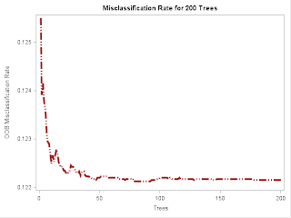
   title "Misclassification Rate for 200 Trees";
   series x=Trees y=VarsToTry8/lineattrs=(Pattern=MediumDashDotDot Tickness=4 COlor=brown);
yaxis label='OOB Misclassification Rate';
run;
title;

"


Subject 1: Do more trees improve classification rate? The plot above shows the classification rate starts to peter to flat ~ 50 trees. After 100 trees, it definitely does not improve any more

Subject 2: "Loss Reduction Variable Importance Report" from random forest often does NOT tell a story about variable importance similar to what you get from other methods


Subject 3: Random Forest Fit Statistics, the Out-of-Bag tree steps


Wednesday, December 26, 2012

K Nearest Neighbor Modeling Using SAS: Proc PMBR

K nearest neighbor modeling (KNN) essentially says: “if you are very similar to k nearest entities, with respect to a list of variables or dimensions, I think it is more likely you will make the decision (as reflected in the target variable) as those K nearest entities make.”
SAS has KNN implementation in its Enterprise Miner. This blog provides code example of the procedure that runs behind Enterprise Miner’s Memory-Based Reasoning Node (MBR),  proc PMBR. Memory based because it simply trains on a training data set and in the same procedure allows you to score another data set. It does not provide a parametric model or rule-set that does generalization or deployment.
Proc dmdb batch data=&indsn(keep=&targetx. &donerx.) dmdbcat=catCR;
   var &donerx. &targetx.;    /*class ;*/
   target &targetx.;
run;
/*you need to run this procedure to create SAS catalog for later processing. It runs very fast even on big data sets with many variables. You may save it to permanent data set if you like*/ 
proc pmbr              /*I think the implied distance is Euclidian*/ 
   data=&indsn.(keep=_numeric_ &targetx.)  dmdbcat=catCR
   THREADS=8  /*the default option is THREADS. You can specify NOTHREADS*/
   OPTIMIZEK /*
  • Specify this option if you want to have data decide # of neighbors. Conceptually it is similar to Cubic Cluster Criterion (CCC)
  • You can clearly specify K=.  Adding WEIGHTED will weight influence of nearest neighbors according to their relative distance to the subject being classfied
  • Large # of neighbors should be balanced against how similarity graduates among the neighbors. You may consider target profiling during the graduation.
  • If your target is binary, selecting even number for K may result in more ties*/ 
    EPSILON=0 /*
  • Minimum allowable distance for a scoring observation to a training observation.
  • If you are not sure how big it should be, leave it at 0.00
  • Depending on collective complexion of the variables listed at VAR statement big Epsilon may give you no neighbors near enough to support classification */ 
   Method=rdtree /*
  • This option determines the data representation that is used to store the training data set and determine the nearest neighbors
  • RDTREE is default
  • Another more data intensive option is SCAN */ 
   out=outx outest=oust;
/*This ends discussion of options at the procedure level. There are several others left out*/ 
   target &targetx.; /*This is statement*/
   var &donerx.;
   /*decision cost= costvar= decisiondata= decvar= priorvar=*/
   score data=temp out=&outdsn.;
run;

General notes

  • As you should heed in conducting distance base classification, scale and the variables being orthogonal to each other are important to the usefulness of your results. Many often conduct standardization and PCA to prepare the data. 'Speciality' treatment may be called upon if your inputs are such as purchase basket, sequence or preference/subjective. Using multi-dimensional scaling is not uncommon. Weighting, however, generally should not be over-done
  • You may consider variable clustering for selection. Some argue that presence of a TARGET should require usual 'variable selection' like building a logistic regression model. Target variable here is little > voting chips. MBR is NOT to maximize separation between 0 and 1
  • Training under this procedure typically does not take very long. Scoring does when distance between observations in the training set and the scoring data set is calculated. This reminds of how proc discrim works when a non-parametric model is built and scored upon
  • You should settle issues such as missing value (surrogates, used-in-distance) and sparcity before engaging the two procedures
  • The scored data set has predicted (voting results from nearest neighbors) score for each observation. You can conduct performance analysis from there (actual vs. predicted…)
Sunday, December 16, 2012

Binning 40 Million Rows on GreePlum, SAS HPBIN


Binning often happens once a model universe is built. A typical credit risk modeler could spend >20% of a project cycle on binning. Let me call this Type I binning application. Another often seen area where analysts bin data is data exploration/ management where the exercise is more ad hoc settlement than analytically premeditated ("Can we just break these 2 billion rows into 10 bins and check out the distribution? I cannot read anything meaningful from the original curve"). Let me call this Type II.
  1. Whether Type I practitioners are going to build models on bigger data is anybody’s Q & A. Or if they do decide to embark on, say, building a random forest model using 40 million *100 input variables, binning may not be considered necessary. Some, regardless of what models to build, are against binning anyway. I believe while domains like credit risk score cards are predicated on binning, many analytical applications involving rich details of big data need to carefully weigh the pro and cons of binning: it is really hard to say whether binning makes signals clearer or not; “binning does not guarantee ‘good’ binning” is a strong argument. It is more about information value of individual data elements, a decision that ought not to be strategic, but more like 'game time decision'
  2. Type II areas, in the past 12 months or so, are quietly orienting towards serious analytical practice. While monitors used to display analytics are getting sharper and sharper, advanced analytics is invading enterprise operations. While profiling remains ‘things to do’ on big data, methods like sequence alignment methods (SAM) are entering batting practice. To align successfully, to large extent, is to bin successfully; analytics is not photography after all. The tallest table I have heard is from a SAS customer who wants to comb through ~20 billion rows several times during a day
SAS did not have a stand-alone procedure for binning until August 2012 when proc HPBIN was introduced as a part of SAS 12.1 HPA (High-Performance Analytics). The focus of this writing is threefold. First is to show syntax example of proc HPBIN. Second is to show how it is like binning a variable that has 40 million rows on a Greenplum cluster.  Last, some new algorithms in the HPBIN procedure
Part One: Syntax of HPBIN (this is procedure has a lot in common with Enterprise Miner)
"
proc hpbin data=&indsn numbin=8 /*supports <=1000*/ computequantile computestats
output=_xin; /*you can write out binned data with or withour replacing original data*/
bucket /* the other 2 methods are winsorized and pseudo_quantile. Pseudo_quantile is one novel way to do quantile binning on big data. Details below */
performance host="&GRIDHOST" install="&GRIDINSTALLLOC";
/*if you have SAS HP grid installed, you can leverage parallel processing there. You can also run locally if you so choose*/
 var cr:;
freq freq1; 
 id acct; 

 /*if ID statement is used, only the ID variable and binned results are included in the output data set. Support multiple IDs. When ID statement is not present, use REPLACE to replace original data*/
 /*code file=code;*/
run;
"
Part Two: Performance Impression

On a Unix server box where SAS Grid Manager governs 32 worker nodes with ~1.5 TB RAM, a credit score variable that has exact 40 million rows resides in a data set that is ~10GB, on a Greenplum cluster. Below are some SAS log details from applying HPBIN to the variable
"
3921  proc hpbin data=&indsn numbin=8 /*pseudo_quantile*/ bucket
3921! out=_xin;
3922      var annual_profit /*cr: os: pur:*/;
3923      id acct_number;
3924  run;

NOTE: Binning methods: BUCKET BINNING .
NOTE: The number of bins is: 8
NOTE: The HPBIN procedure is executing in the distributed computing environment with 32 worker
      nodes.
NOTE: The data set _XIN has 40000000 observations and 2 variables.

NOTE: PROCEDURE HPBIN used (Total process time):
      real time           14.41 seconds
      cpu time            2.25 seconds

"
  1. If today's top big UNIX boxes are Ph.D., this box is more like undergraduate freshman. Still, it is a decent BIG box. Unless your application is like fraud detection, this speed is acceptable
  2. There was 2 concurrent jobs running at the same time.
  3. While I know the performance is not very linear with the # of rows, under the same condition, if you bin 400 million rows on this variable, your total real time likely will be < 1 minute
  4. The gap between CPU time and Real time is significant, indicating some data movement
  5. I have not had chance to test this on Hadoop. I ran some SAS HPA work on Hadoop clusters. I suspect the performance there will be comparable with this box. You just need to reset your libname
Part Three: Something novel

In quantile binning where sorting is very particular, tall variables can pose enormous computation challenges. Tall variables in big data certainly get much taller. Procedure syntax appears very simple but the sorting algorithm in the background is complex (Winsorization does not get much better). I don't want to turn this writing into manual reading or technical training. Just a brief: " The pseudo–quantile binning method in the HPBIN procedure can achieve a similar result with far less computation time...." You can indulge in more details when you get to read SAS HPA documents. Important is this may give you a good glimpse on how SAS tackles big data computation: leverage its industry-dominant strength in algorithm research, innovation and implementation.


Sunday, December 9, 2012

Stochastic Gradient Boosting Modeling in SAS: A Procedure Example

Some of my friends are pretty experienced modelers. They have asked me if SAS has stochastic gradient boosting (SGB) capabilities. I told them Enterprise Miner has had it for ~8 years.  But they told me using SAS Enterprise Miner makes them appear ...junior level. This post shows one procedure syntax example of SGB

Here is the SAS code (IF data elements look like yours, that is pure coincidence)

%macro treeboost2;
proc treeboost data=&indsn

 /*INMODEL: use data= to build it or use inmodel= to read in existing models*/

  CATEGORICALBINS=6
  INTERVALBINS=35
  /*this idea is similar to coarse binning in credit scoring card*/

  EXHAUSTIVE=100 /*could be bigger*/
  INTERVALDECIMALS= MAX /*Trees are decimal sensitive*/
  leafsize=2
  Iterations=1000 /*maxbranch= maxdepth=  + several other options*/
  Mincatsize=2
  missing=useinsearch /*distribute,*/
  seed=989795
  SHRINKAGE=0.1 /*If you are grounded in SGB, you know its role. default  =0.2.   Be gradual, be very gradual,if you want to boost well*/
  SPLITSIZE=20  /*split a node only when it contains at least number Observations. The default value is twice the size of the vaue specified in LEAFSIZE=   */ 

Input &select_s /*If you don't differentiate, it treats numeric as interval and character variables as categorical--class variables*/
   /INTERVALDECIMALS=5 /*MAXBRANCES=*/
    MINCATSIZE=2
    MISSING=useinsearch /*distribute bigbranch*/
    order=descending /*sorting order of oridnal*/;  

  Target &targetx. /level=binary;
  save FIT=fit IMPORTANCE=imp MODEL=mdl RULES=rules;
  /*score data=score out= outfit=outfit prediction*/
  SUBSERIES longest; /*Best iteration=100*/
  /*The SUBSERIES statement specifies how many iterations in the series to use in the model. For a binary or interval target, the number of
  iterations is the number of trees in the series. For a nominal target with k categories, k > 2, each iteration contains k trees. The following
        options are mutually exclusive.*/;

run;
quit;
%mend treeboost2;

"

I am not going to visualize and compile the performance results as Enterprise Miner does. Here are some SAS log details

"
NOTE: Assuming numeric variables have INTERVAL measurement level, and character variables have NOMINAL.

NOTE: 1671263 kilobytes of physical memory.

NOTE: Will use 168252 out of 168252 training cases.

NOTE: Using memory pool with 410163200 bytes.

NOTE: Passed training data 5000 times.

NOTE: Current TREEBOOST model contains 1000 trees.

NOTE: Training used 15327976 bytes of work memory.

NOTE: The data set WORK.FIT has 1000 observations and 11 variables.

NOTE: The data set WORK.IMP has 31 observations and 4 variables.

NOTE: The data set WORK.MDL has 141996 observations and 4 variables.

NOTE: The data set WORK.RULES has 20805 observations and 7 variables.

NOTE: Current TREEBOOST model contains 1000 trees.

NOTE: There were 168252 observations read from the data set LOCALX.DLQ_ACT_MODELDEV.

WHERE RANUNI(987282)<=0.1;

NOTE: PROCEDURE TREEBOOST used (Total process time):

real time 12:22.92

cpu time 11:55.98"

 
There are another ~1/3 statements and options not shown. This is quick view. Enjoy. My local PC has 32 GB RAM. This post does not focus on processing speed so I just took 10% random sample.